

Read the first chapter
The whole of chapter one, free. About 9 min. Turn the pages with the arrows, your keyboard, or a swipe.
Chapter 1
Market Data for Simulation Inputs
A backtest that “looks right” often hides a quiet failure: your input data drifts out of sync by a few minutes, your corporate actions get applied twice, or your bars get stitched together across trading halts without you noticing. Those problems don’t always crash your pipeline. They just make the simulated strategy slightly too good, then slightly wrong out of sample, and you end up chasing ghosts.
Talia, 34, a prop trader who runs backtests daily, learned this the hard way. One afternoon her equity curve jumped exactly when she expected it to fade. The change wasn’t in the model logic; it was in the data. The vendor had updated the corporate action file, and her script had pulled the new split factors but left the old dividend adjustments in place. The simulation started trading on adjusted prices that no longer matched the volume and timestamp conventions the rest of her code assumed.
This chapter shows you how to clean, align, and transform raw market data into simulation-ready inputs you can trust. You’ll end up with a repeatable process that produces a consistent time index, correct price/return series, and feature columns that stay aligned with the trading logic in your backtest or agent-based simulation. You’ll also learn how to catch the specific failure modes that create “too-good” backtests: duplicate adjustments, time-zone mismatches, and silent bar construction errors.
Input Sanity Checklist: cleaning, aligning, and transforming without guessing
The core move is to stop treating data prep as a one-off script. You need a checklist you run every time you build a dataset, and you need rules that translate raw vendor fields into simulation primitives: a clean timestamp, an orderable price series, and a return series (or state variables) that align with your execution model. Think in terms of invariants: if an invariant breaks, you fix the data before you run the model.
Use this Input Sanity Checklist for every instrument and every dataset version. It focuses on the three things that break simulations most often: time alignment, corporate actions, and bar construction.
1. Lock the time axis first (timestamp hygiene). Convert every feed you use - trades, quotes, OHLCV bars, corporate actions - into one canonical timezone (usually UTC) and one canonical bar boundary rule. Then verify that your final index is monotonic and has no unexpected gaps. If you simulate minute bars, you want exactly one row per minute per instrument between start and end, or you want explicit markers for missing minutes.
2. Apply corporate actions once, in the right order. Adjust prices for splits and dividends exactly once, using the vendor’s official action effective dates. For OHLCV bars, apply adjustments to all OHLC fields consistently, and decide what you do with volume (many pipelines scale volume by split factors but keep dividend effects out of volume). Your invariant: adjusted prices should reconcile with unadjusted prices via the cumulative adjustment factor.
3. Choose one price definition for execution and stick to it. Decide whether your strategy trades on the bar’s open, close, or a synthetic “next-bar open.” Convert your OHLC into the exact input your execution model expects. For example, if you run “enter at next bar open,” you must shift the features and labels so that the prediction at time t maps to the execution at time t+1. Mis-shifts create look-ahead bias without any obvious error.
4. Rebuild returns from the same adjusted price series. Compute returns only after you’ve finalized adjusted prices. If you compute returns earlier and then adjust prices later, you break the math. Your invariant: the return series should satisfy the identity \[ r_t = \frac{P_t}{P_{t-1}} - 1 \] (or log returns, if you use them) using your final adjusted price series.
Here’s a concrete example you can apply immediately. Suppose your vendor provides daily OHLCV and a separate corporate actions file. You ingest both into a dataframe. First you standardize timestamps: you make each daily bar timestamp represent market close in UTC (or market open - just be consistent with your execution rules). Next you compute an “adjustment factor” column from the corporate actions file and apply it cumulatively to the daily OHLC. Then you compute returns from the adjusted close. Finally you create shifted columns for labels: if your strategy predicts tomorrow’s return, you shift the return target by one day and you keep all features unshifted.
If you also use intraday data (quotes or trades) to build features like spread or midprice, you align those features to the bar boundaries after cleaning. For minute bars, you construct midprice from the best bid and ask at each minute boundary, then forward-fill only within the bar grid you already validated.
The practical trick: you don’t “clean until it runs.” You clean until the invariants pass. Invariants are the difference between “my script works on this dataset” and “my simulation inputs are consistent across revisions.”
Putting it into practice: build a simulation-ready dataset for minute bars
Let’s walk through a realistic scenario with Talia’s daily workflow, but keep it generic enough to run on your own setup. Assume you want to run a simulation on 1-minute bars for one equity. You have:
• A minute OHLCV file (with timestamps) - A corporate actions file (splits and dividends with effective dates) - Optional bid/ask quotes if you compute spread features
Your goal: produce a dataframe where row t corresponds to the minute bar that starts at timestamp t, and every feature at t only uses information available up to that minute boundary.
1. Ingest and standardize timestamps. Read the minute OHLCV and corporate actions into memory. Convert timestamps to UTC. Choose a bar boundary convention: for minute bars, set the bar timestamp to the minute start time (e.g., 14:30:00 UTC). Expected outcome: your index becomes a regular grid with one row per minute for trading minutes.
2. Validate the time grid before you touch prices. For each trading day, count minutes and compare against what you expect from your trading calendar rules. If you find missing minutes, decide whether to drop the day, fill gaps, or mark gaps with a flag. Expected outcome: you prevent “partial day” contamination that can make returns look smoother than they should.
3. Build a cumulative adjustment factor and apply once. From the corporate actions file, compute a cumulative adjustment factor for each timestamped bar. Apply the factor to OHLC consistently. Decide on volume handling: for split-only adjustments, multiply volume by the split factor; for dividends, keep volume unchanged. Expected outcome: after adjustment, adjusted prices match the relationship between pre- and post-adjustment by your factor.
4. Create the execution price and shift features correctly. Pick your execution price. If you simulate “enter at next minute open,” set execution price at time t+1 using the open from the shifted series. Then shift your label accordingly: if the label is next-minute return, compute it from adjusted close (or open-to-open, depending on your model) and align it so that features at t map to label at t+1. Expected outcome: you eliminate look-ahead bias caused by accidental alignment.
5. Compute returns from the final adjusted series. Compute log returns or simple returns using the adjusted price series. Expected outcome: no NaNs except at the first bar (or after missing days you flagged).
6. Add a “sanity meta” output. Write a small summary table that includes counts: number of bars, number of corporate actions applied, number of missing minutes, and max/min adjustment factors. Expected outcome: when you rerun later, you can diff the summary and catch silent pipeline changes.
Quick checklist (run it every time you rebuild inputs):
• Confirm timestamps are UTC and monotonic - Ensure your minute grid has exactly one row per expected bar boundary for trading minutes - Apply splits and dividends once using effective dates; adjust OHLC consistently - Compute returns from the adjusted price series only - Align features and labels with your execution rule (e.g., shift by one bar for next-bar execution) - Produce a small run summary so you can detect pipeline drift
If you also compute features from quotes (spread, midprice, order imbalance), apply the same timestamp hygiene and grid validation. Then resample quotes into minute buckets using a consistent rule (e.g., last observation in the minute, or the observation at the minute boundary). Your invariant stays the same: every minute feature row must reflect only data available up to that minute boundary.
What to watch for: common mistakes and how to fix them
Even with a checklist, you’ll hit edge cases. The goal is to recognize the pattern quickly, fix it at the data level, and rerun the invariants before you touch model code.
Duplicate corporate action application What happens: you apply split factors once in your price-adjustment step, then your returns step (or a second script) applies them again. The symptom: adjusted prices jump more than they should around the effective date, and the adjustment factor series shows discontinuities that don’t match the action file. Do this: confirm you apply corporate actions exactly once by logging the cumulative adjustment factor you use and comparing it to the vendor’s “post-adjustment” reference if available. Also ensure your pipeline never re-adjusts an already-adjusted price column. Not this: compute returns from an “adjusted close” you created earlier, then re-run a price adjustment transformation on the same dataframe “just to be safe.”
Time-zone mismatch and bar-boundary drift What happens: your OHLCV timestamps come in local exchange time, your corporate actions use UTC, and your feature engineering assumes UTC. The symptom: corporate actions get applied to the wrong bar, and your execution price shifts by a minute or more. That kind of misalignment can still produce a smooth curve, which makes it harder to detect. Do this: standardize timestamps immediately after ingestion. Then apply corporate actions using the same canonical timezone and bar boundary convention you use for your simulation grid. Not this: adjust timestamps after you’ve already resampled quotes or constructed bars, because you’ll shift the data without updating the resampling logic.
Silent missing bars treated as valid market What happens: a vendor occasionally omits a few minutes (or a day) without warning. If you forward-fill without marking gaps, your returns can look artificially stable and your execution model can “trade through” periods that never existed in the input. The symptom: your bar count per day doesn’t match your expected trading minutes, but your model still runs. Do this: detect missing minutes during the time-grid validation stage and either drop the affected day or set a gap flag and force your strategy to skip trading those bars (depending on your simulation rules). Not this: fill gaps with the last close and keep everything else the same. You’ll create price paths that the market never produced.
These fixes all land in the same place: you protect the invariants. If time alignment breaks, you don’t patch it with shifting tricks later. If corporate actions break, you don’t “smooth” the returns. You correct the transformation so the dataset represents the market sequence your model assumes.
A good dataset doesn’t just “run.” It passes the same sanity checks every time you rebuild it, even after you update vendor files or change feature code. When you treat data prep like part of the model - versioned, validated, and invariant-driven - you stop guessing why backtests change and you start improving the actual trading logic that sits on top.
End of chapter one. 7 more chapters in the full book.
Swipe or use the arrows to turn the page


What's inside: 8 chapters
- 1. Market Data for Simulation Inputs
- 2. Choosing a Market Microstructure Model
- 3. Calibrating Stochastic Price Dynamics
- 4. Backtesting Agent Strategies with Walk-Forward
- 5. Designing Agent Behaviors and Rules
- 6. Validating Simulations with Statistical Tests
- 7. Stress Testing with Adversarial Scenarios
- 8. From Simulation to Live Trading Deployment
About this book
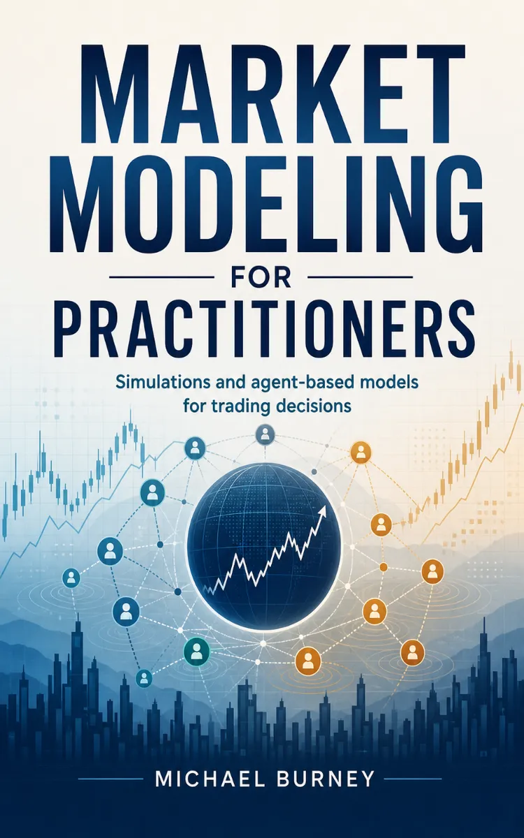
"Market Modeling For Practitioners" is a finance book by Michael Burney with 8 chapters and approximately 16,320 words. Trading-focused market modeling using simulations and agent-based models.
This book was created using Inkfluence AI, an AI-powered book generation platform that helps authors write, design, and publish complete books. It was made with the AI Ebook Generator.
Frequently Asked Questions
What is "Market Modeling For Practitioners" about?
Trading-focused market modeling using simulations and agent-based models
How many chapters are in "Market Modeling For Practitioners"?
The book contains 8 chapters and approximately 16,320 words. Topics covered include Market Data for Simulation Inputs, Choosing a Market Microstructure Model, Calibrating Stochastic Price Dynamics, Backtesting Agent Strategies with Walk-Forward, and more.
Who wrote "Market Modeling For Practitioners"?
This book was written by Michael Burney and created using Inkfluence AI, an AI book generation platform that helps authors write, design, and publish books.
How can I create a similar finance book?
You can create your own finance book using Inkfluence AI. Describe your idea, choose your style, and the AI writes the full book for you. It's free to start.
Write your own finance book with AI
Describe your idea and Inkfluence writes the whole thing. Free to start.
Start writingCreated with Inkfluence AI


