

Read the first chapter
The whole of chapter one, free. About 10 min. Turn the pages with the arrows, your keyboard, or a swipe.
Chapter 1
Order Book Microstructure Basics
A single limit order can move the market more than you expect, even if nobody “buys” it right away. If you’ve ever watched the best bid lift by a tick while the tape looked calm, you already saw the real mechanism: price forms from queues of resting orders and the trades that consume them. The order book does not just “show liquidity”; it manufactures the next price level by revealing where traders are willing to wait and how quickly incoming market orders eat through that willingness.
For practical trading, the problem isn’t that you don’t know the definitions of bid, ask, and spread. The problem is that you can’t connect those definitions to what you can measure and trade: how much depth sits in each price level, how that depth changes as orders arrive and cancel, and how your own orders affect the queue you’re joining. This chapter gives you a concrete way to read that queue behavior directly from limit orders and trades, so you can reason about price, liquidity, and execution friction without hand-waving.
After you finish, you’ll be able to (1) translate an order book snapshot into queue pressure, (2) map a sequence of trades into which price levels got consumed, and (3) run “what-if” checks before you place an order so you don’t guess whether you’ll fill or get left behind.
Set the context: why price, liquidity, and queues depend on limit orders and trades
Talia, 34, spent years on the trading floor watching order flow decide whether a move held or reversed. When she shifted into quant research, she brought a blunt takeaway with her: the chart price you see is the result of mechanical consumption, not a clean signal of “value.” In liquid markets, most of the time the market doesn’t reprice because everyone suddenly changed their mind; it reprices because resting limit orders at the current best prices get hit, canceled, replenished, or skipped.
That matters because liquidity you can’t quantify still acts like a force. If depth at the best ask vanishes when the market approaches it, your market order pays more than you expected. If a queue thickens just outside the spread, your limit order might fill faster than your backtest suggests - or not fill at all if cancels spike. You need a way to tie together three things that traders often treat separately: the price path (from trades), the available liquidity (from resting orders), and the queue dynamics (from how trades walk the book).
This chapter solves that connection problem with a single working model: Queue-to-Price Compass. You won’t treat the order book as a static ladder of numbers. You’ll treat it as a set of queues, where each trade (and each cancellation you infer) advances the “compass needle” from one price level to the next until the next incoming order finds enough resting volume to stop the walk.
By the end, you’ll be able to look at a live book (or a historical reconstruction), mark which levels get consumed by trades, estimate queue pressure from changes in depth, and make execution decisions that match those mechanics.
How it works: the Queue-to-Price Compass for order-book-driven price formation
The core idea is simple: price changes when incoming marketable orders consume resting limit orders at the current best prices. Liquidity is what those resting orders offer, and queue dynamics govern how far the consumption travels before it runs out.
To make this usable, you need a consistent mapping from “what the book shows” to “what the tape does.” The Queue-to-Price Compass gives you that mapping by tracking three measurable objects at each timestamp (or event time):
1) the best prices (best bid and best ask), 2) the resting volume at those prices (the queue sizes), 3) the incremental changes in those volumes as trades execute and orders cancel.
Here’s the practical technique, with concrete rules you can implement.
1. Define the queue you care about: start from the best price you expect to interact with. If you plan to buy, focus on the ask-side queues: the best ask and the nearby levels above it. If you plan to sell, focus on the bid-side queues at and below the best bid. This keeps your analysis aligned with your execution path.
2. Compute “queue depth gradients” around the best price. Take the resting volume at the best price (say, best ask level \(p\)) and compare it to the next level (say, \(p+\Delta\)). A large jump means the book can absorb a small number of shares without forcing price up; a shallow ramp means a walk through levels is likely. You can compute this with a simple ratio like \( \text{Depth}_{p+\Delta} / \text{Depth}_{p} \) or a difference \( \text{Depth}_{p+\Delta} - \text{Depth}_{p} \).
3. Translate trades into “queue consumption” at those price levels. When you see an executed trade at price \(p\), attribute its volume to the queue at that price. Then update the remaining queue depth at \(p\) by subtracting the executed size. If your data includes full depth updates, you can verify directly; if it doesn’t, you can still infer consumption by matching trade prices to the last known best levels.
4. Estimate cancellation pressure as “depth disappears without trades.” If depth at a price level drops while no trade prints at that level, you attribute the reduction to cancellations (or order re-pricing). This step matters because cancellations can make a book thin exactly when you arrive, turning a “should fill” into a “miss.”
A concrete example: suppose the best ask is 100.00 with 800 shares resting, and the next ask level 100.01 has 200 shares. You submit a marketable buy of 900 shares. The first 800 shares consume the 100.00 queue, so the next 100 shares must consume 100.01. Your average execution price rises because the queue at 100.01 is shallow. If later you observe that 100.01 depth drops from 200 to 20 right before you act (without any 100.01 trades printing), you just saw cancellation pressure that will worsen your fill.
The compass part comes from combining those steps into a directional expectation: given the current queue sizes and their changes, where will the next trade-driven price stop if you keep consuming in the same direction? You can answer that with a small “walk the book” calculation each time you consider an order.
Putting it into practice: a realistic scenario with expected outcomes and a checklist
Use Talia’s transition workflow mindset: she doesn’t start with a thesis; she starts with an order book capture and an execution plan. Here’s a scenario you can replicate with your own data feed or backtest reconstruction.
Assumptions (grounded, so you can swap in your own numbers): - Tick size \(\Delta = 0.01\). - You plan a buy using immediate-or-cancel logic (or a marketable limit that executes immediately up to its limit). - Your data feed gives you: best bid/ask, depth at each level for a few ticks, and trade prints with price and size.
Step-by-step execution using the Queue-to-Price Compass
1. Snapshot the book and extract the ask-side queues. At time \(t\), you observe: - Best ask: 100.00 with 800 shares - Next ask: 100.01 with 200 shares - Next ask: 100.02 with 600 shares Expected outcome: the book can absorb up to 1000 shares with only a small price jump, then it likely pushes to 100.02 if more demand arrives.
2. Compute a simple walk for your intended size. You plan to buy 1100 shares marketably (crossing the spread). - Consume 800 at 100.00 → remaining 300 - Consume 200 at 100.01 → remaining 100 - Consume 100 at 100.02 → remaining 0 Expected outcome: you’ll trade 800 at 100.00, 200 at 100.01, and 100 at 100.02. Your average price will sit between 100.01 and 100.02, closer to 100.01 because most volume hits 100.00.
3. Check for cancellation pressure right before you send. Within the last 200 milliseconds, you notice: - 100.01 depth dropped from 200 to 50 - No trades printed at 100.01 during that interval Expected outcome: your earlier walk breaks. With only 50 shares at 100.01, your 1100-share buy will consume: - 800 at 100.00 → remaining 300 - 50 at 100.01 → remaining 250 - 250 at 100.02 (instead of 100 at 100.02) Your average price worsens because the queue you counted on got pulled.
4. Set your limit price (if you use a marketable limit) from the compass, not from gut feel. If your maximum acceptable average price is 100.015 (you pick this from your P&L tolerance and typical slippage regime), you translate that into a worst-case walk scenario: assume the shallowest nearby queue after cancellations and compute the resulting average. Expected outcome: you either (a) place a limit high enough to execute the full size under the worst-case walk, or (b) reduce size so you execute only where the compass predicts the fill will stop.
5. After execution, verify queue consumption against trades. Once your order completes, compare: - how many shares executed at each price level, - whether the trade prices moved exactly along the levels you predicted, - whether any unexpected price jump occurred (which usually signals either hidden liquidity, a different depth snapshot than you used, or sudden new arrivals that changed the book).
If you do this consistently, you stop treating execution as “slippage noise” and start treating it as a direct consequence of queue dynamics you can read.
Quick checklist (use this before you hit send)
• Capture best ask and the next 2-3 ask levels with their resting share counts. - Walk the book for your intended size and compute the expected level-by-level consumption. - Detect cancellation pressure by checking depth drops at levels without corresponding trade prints. - Translate the worst-case walk into a limit price or a reduced order size. - Post-trade, reconcile executed price levels with your predicted consumption path.
That’s the mechanical loop: read queues → predict the walk → place order → verify consumption.
What to watch for: mistakes and edge cases that break the compass
If you rely on the compass without accounting for common failure modes, you’ll get blindsided. Here are the ones that show up fastest in real trading.
Hidden liquidity and “non-displayed” size
When you see depth at the best ask that looks thin, you may assume your marketable buy will walk up quickly. But many venues and feeds include only displayed depth; additional liquidity can sit hidden, replenishing the queue right when you think it will empty.
Do this: Use your post-trade reconciliation to detect systematic mismatches. If you repeatedly predict consumption into 100.02 but executions often stop at 100.01, your feed likely missed non-displayed orders. Adjust your model by widening the depth window (next levels) and treating displayed depth as a lower bound, not the full queue.
Not this: Treat displayed depth as the entire queue and lock your limit price tightly to a single snapshot. That assumption breaks in venues with meaningful hidden liquidity.
Queue changes caused by your own order flow
If you place multiple orders back-to-back, your earlier order can change the book before your later one arrives. Your own marketable buys consume queues and can trigger cancellations or re-posting at new prices. The compass then interprets those changes as “market” dynamics when they’re partly self-inflicted.
Do this: Separate “impact” from “signal.” When you study a strategy, run it in a paper environment first or use a replay where you can label which trades belong to your algorithm. At minimum, measure whether the depth you read right before order submission changes in a way correlated with your own executions.
Not this: Build a model that treats depth changes as exogenous while ignoring that your own order consumption is part of the queue dynamics you’re modeling.
Stale snapshots and event-time misalignment
Your queue-to-price mapping assumes the depth snapshot matches the event time of the order. If your code reads the book at \(t\) but sends the order at \(t+50\) milliseconds, the queue can change through cancellations, new limit placements, or trade prints you didn’t observe. That turns the compass into a compass pointing at the wrong map.
Do this: Timestamp everything. Align your book snapshot timestamp with the order submission timestamp and the first trade you observe. If you backtest, use event-time order book reconstruction rather than bar-based snapshots. Expect to see large execution errors when you align to coarse time buckets.
Not this: Use a “best bid/ask at the last mid” feature without accounting for latency or event ordering. Your fills will drift because the underlying queues drift.
A final edge case worth respecting: the compass works best when you keep the consumption direction consistent (buy-to-ask, sell-to-bid). If you alternate rapidly or use large orders that span multiple price levels, the queue you “walk” through can change mid-walk due to new arrivals and cancellations. In that case, you still can use the compass, but you must shorten the horizon and refresh the walk more frequently.
Price, liquidity, and queue dynamics aren’t separate stories on the screen. They’re one story told by limit orders and trades, with cancellations acting like punctuation. Once you train yourself to read “where the walk stops” from the queue, your execution decisions stop being guesses and start being mechanical expectations you can test and refine.
End of chapter one. 7 more chapters in the full book.
Swipe or use the arrows to turn the page


What's inside: 8 chapters
- 1. Order Book Microstructure Basics
- 2. Bid-Ask Spread Decomposition
- 3. Market Impact and Execution Costs
- 4. Designing a VWAP/TWAP Participation Plan
- 5. Modeling Limit Order Placement
- 6. Adverse Selection with Trade Signatures
- 7. Estimating Volatility from Microstructure Noise
- 8. Case Studies: From Backtest to Live Fills
About this book
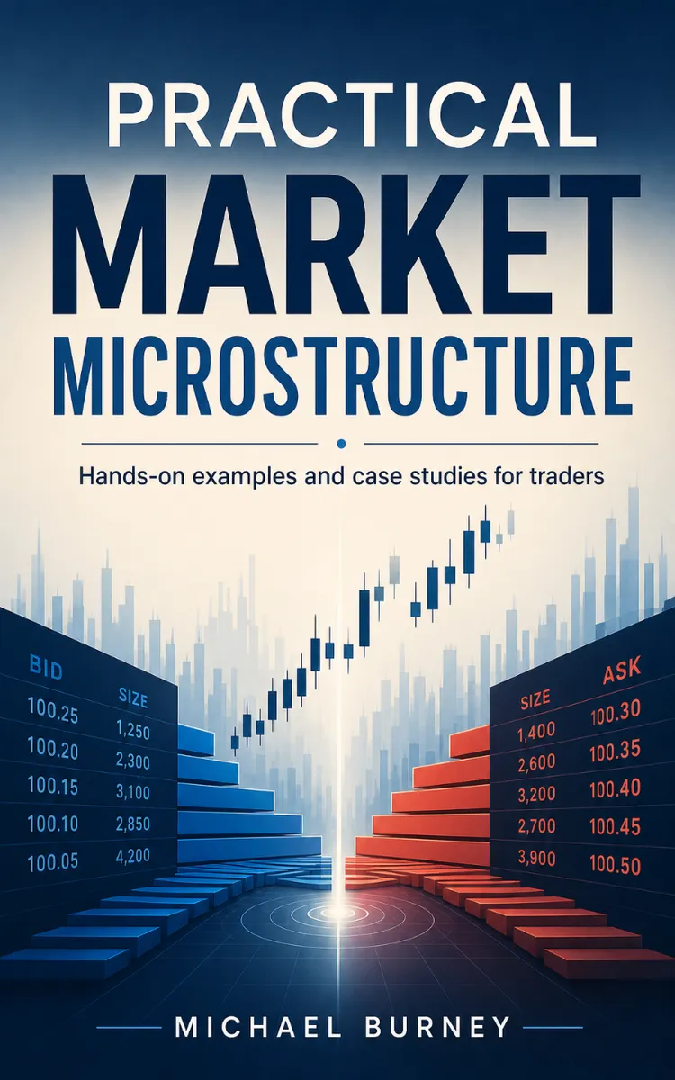
"Practical Market Microstructure" is a finance book by Michael Burney with 8 chapters and approximately 18,268 words. Market microstructure concepts applied through examples and case studies.
This book was created using Inkfluence AI, an AI-powered book generation platform that helps authors write, design, and publish complete books. It was made with the AI Ebook Generator.
Frequently Asked Questions
What is "Practical Market Microstructure" about?
Market microstructure concepts applied through examples and case studies
How many chapters are in "Practical Market Microstructure"?
The book contains 8 chapters and approximately 18,268 words. Topics covered include Order Book Microstructure Basics, Bid-Ask Spread Decomposition, Market Impact and Execution Costs, Designing a VWAP/TWAP Participation Plan, and more.
Who wrote "Practical Market Microstructure"?
This book was written by Michael Burney and created using Inkfluence AI, an AI book generation platform that helps authors write, design, and publish books.
How can I create a similar finance book?
You can create your own finance book using Inkfluence AI. Describe your idea, choose your style, and the AI writes the full book for you. It's free to start.
Write your own finance book with AI
Describe your idea and Inkfluence writes the whole thing. Free to start.
Start writingCreated with Inkfluence AI


